Category Archives: Cloud Services

AWS Interconnect Multicloud Just Added Azure — Here’s What That Actually Buys You

A few years ago, if you wanted a private link between an AWS VPC and a workload sitting in another cloud, the honest answer was: go find a colo. You’d order a cross-connect, provision a router on each side, stand up a VPN or a pair of Direct Connect circuits, and then hand-configure BGP sessions and hope the failover behaved the way the runbook said it would. It worked, but it was a project, not a feature — weeks of lead time, and yours to operate for as long as the link existed.

AWS Interconnect for MultiCloud setup

That’s the backdrop for why AWS Interconnect – multicloud matters, and why the last twelve months of announcements are worth actually reading instead of skimming. In September, AWS put Microsoft Azure into public preview as the third cloud to adopt the interconnect specification, a month after Oracle Cloud Infrastructure crossed into general availability. Between those two announcements sits a genuinely different way of thinking about cross-cloud networking, and also a few gaps that I’d want a client to understand before they bet a production DR path on it.

What you’re actually provisioning

Strip away the marketing language and Interconnect is a managed Layer 3 private connection between your AWS environment and a partner cloud, with the physical and routing complexity abstracted into a single object. On the AWS side, the attach point is always a Direct Connect Gateway — that’s the one thing you touch. On the partner side it’s a CSP router, and AWS and the partner negotiate an Activation Key between them: one party creates the request, the other accepts it, and provisioning happens automatically on both sides. You never see a BGP session config or a VLAN tag.

Underneath that single logical object, AWS builds four physical connections across at least two separate buildings with independent power and networking, load-balanced with ECMP so that a device or facility failure doesn’t take the link down — only one of the four paths needs to survive. Every physical hop between an AWS router and a partner router runs IEEE 802.1AE MACsec, and it’s not optional: if the encrypted session drops, traffic stops, full stop, rather than falling back to anything unencrypted. That’s a reasonable default for anyone crossing a cloud boundary, though it does mean an encryption negotiation failure is now also a connectivity failure, which is worth knowing before your first 3am page.

AWS Interconnect.

The diagram above hides a detail that’s easy to miss in the docs: a Virtual Private Gateway or Transit Gateway can only reach an Interconnect that’s local to its own Region. If you want any Core Network Edge in your Cloud WAN global network to reach any Interconnect anywhere, attached to the same Direct Connect Gateway, you need Cloud WAN in the picture. For a single-region pilot that distinction doesn’t matter. For a multi-region architecture it’s the difference between one interconnect per region pair and one global fabric, and it changes how you’d design the topology from day one.

The three-provider board, as of this month

Here’s where things actually stand, because “multicloud” has meant three different maturity levels depending on which partner you’re asking about:

  • Google Cloud — generally available since April 2026, the longest-running and most mature pairing. It spans five region pairs (US East N. Virginia, US West N. California, US West Oregon, Europe London, Europe Frankfurt), scales to 100 Gbps, and carries a published SLA on the AWS side.
  • Oracle Cloud Infrastructure — reached GA in July 2026 after a preview that started in May, but only in a single region pair: us-east-1. If your OCI footprint isn’t in N. Virginia, this doesn’t help you yet.
  • Microsoft Azure — entered preview at the end of August 2026, covering four regions (US East N. Virginia, US West N. California, Asia Pacific Sydney, Europe Frankfurt). Preview means no SLA and, as far as I can tell from the announcement, no finalized pricing on the Azure side either.
Timeline

Laid out on a timeline like that, the pattern is obvious: AWS is running the same playbook with every partner — preview in a handful of regions, then GA once the physical build-out and pricing catch up. If you’re planning around Azure connectivity, treat it the way you’d treat any preview service touching production traffic: fine for a proof of concept, not something I’d put in a DR failover path yet.

Why this is an open spec and not just an AWS product

The mechanism behind all three partnerships is the same open specification for network interoperability, published under Apache 2.0 back when Google Cloud joined at re:Invent 2025. Any cloud provider can implement it and become an Interconnect partner without a bespoke bilateral integration each time — which is exactly what happened with OCI and now Azure, both adopting the same spec rather than AWS building three separate point-to-point products.

Forrester’s Lee Sustar has been fairly blunt about the strategic reading: this lets AWS use its market position to push the industry toward its interconnect model as the de facto standard, rather than a neutral committee-driven one. I don’t think that reading is wrong, exactly, but I’d add a second layer to it. Once three of the largest providers are running the same API surface, walking it back gets expensive for everyone involved — including AWS. Azure’s own networking leadership described wanting to extend this model past a single cloud-to-cloud relationship, which suggests they’re not treating this purely as playing along with an AWS-authored spec. Whether that turns into genuine multilateral governance or stays “AWS writes the spec, everyone else implements it” is worth watching over the next year, not something settled by this announcement.

What changes for the team actually running the network

If you’ve built cross-cloud connectivity the old way, the operational shift is real. You’re not configuring BGP timers or ordering physical cross-connects — you pick a Region, a partner, and a bandwidth tier, and the object shows up. Bandwidth is elastic after the fact too: you can scale it up or down from the console without a re-provisioning cycle, which matters if your cross-cloud traffic has a seasonal or campaign-driven shape.

Monitoring comes bundled rather than bolted on. Every Interconnect includes a CloudWatch Network Synthetic Monitor for round-trip latency and packet loss at no extra charge, plus a bandwidth utilization metric you can alarm on before you hit a ceiling. The one gap: AWS’s own docs note that the Network Health Indicator feature isn’t supported on Interconnects yet, so you’re relying on the synthetic probe and utilization metric rather than a single composite health signal. Worth knowing if your ops team is used to that indicator elsewhere in the Direct Connect family.

Pricing, and where the savings are real

The pricing model itself is refreshingly simple: a flat hourly rate based on bandwidth tier and how “local” the region pairing is, with zero per-gigabyte data transfer charges. A 10 Gbps Interconnect between us-east-1 and Google Cloud’s paired N. Virginia region runs about $12.33 an hour — call it $9,000 a month if you leave it running continuously, though you’d size and schedule it to your actual traffic pattern rather than leaving a static circuit up around the clock. Since May 2026, every account also gets one free local 500 Mbps interconnect per Region, which is a genuinely useful way to validate connectivity before you commit real budget.

The no-egress-fee structure is where this actually pays for itself. If you’re moving tens of terabytes a month between clouds — database replication, backup pipelines, analytics pulling from a partner cloud’s data lake — standard internet egress adds up fast, and a fixed hourly bandwidth charge starts looking cheap by comparison well before you hit the circuit’s ceiling. If your cross-cloud traffic is bursty and small, the math is much less compelling, and you’re probably fine on a VPN.

Where I’d actually reach for this, and where I wouldn’t

I’d use Interconnect – multicloud today for exactly the kind of workload it was clearly built for: steady, high-volume data movement between AWS and Google Cloud where the region pairing lines up, or between AWS and OCI if your Oracle footprint genuinely lives in us-east-1. Cross-cloud DR replication, bulk ETL, anything where the alternative was going to be a Direct Connect circuit into a colo anyway — this removes real operational weeks from that project.

I’d be more cautious treating it as a wholesale replacement for a broader multicloud networking fabric. It’s a managed point-to-point bridge between specific region pairs on specific partner clouds, not a global mesh, and OCI’s single-region availability is a real constraint if your estate is more spread out than that. The Azure leg is a preview product without a finalized SLA, so I wouldn’t route anything customer-facing over it until GA lands — and given the Google and OCI timelines, that’s probably a late-2026 or 2027 conversation, not a Q4 one.

The specification being open is the part I’d keep an eye on longer term. If a fourth or fifth provider adopts it, or if governance shifts away from “AWS publishes, others implement,” this stops being an AWS product with two guest stars and starts looking like an actual industry convention for how clouds talk to each other. That’s the more interesting story, and it isn’t finished yet.
Amazon ECS Closes Its Zombie Node Gap — Sort Of

An EC2 instance can be running, passing its own status checks, and billing you same as always. It can also be completely useless to ECS. An EBS volume degrades. A host hits a thermal event. Some network path glitches. The ECS agent quietly stops talking to the control plane, and the instance isn’t dead — it’s a zombie: present in your account, absent from anything that actually matters. Until August 24, ECS had no clean, structured way to tell you that had happened.

ECS Faulty Nodes Handling!

What actually shipped

AWS announced that ECS now folds agent connectivity into its structured container instance health checks, and, more importantly, automatically remediates it on two of three compute options.

The signal itself isn’t new. ECS has always exposed an agentConnected flag on container instance state-change events, and AWS has spent years walking customers through wiring up EventBridge, SQS, and Lambda just to catch it. What’s new is that agent connectivity now joins CONTAINER_RUNTIME, ACCELERATED_COMPUTE, and DAEMON as a proper health check type feeding into a container instance’s overallStatus — the same object you already pull with:

aws ecs describe-container-instances \
  --cluster my-cluster \
  --container-instances <container-instance-id> \
  --include CONTAINER_INSTANCE_HEALTH

It watches for the class of failure that’s hardest to catch from inside the instance itself: EBS volume degradation, host thermal events, or network connectivity failures that sever the agent’s line to the control plane without necessarily touching the container runtime or the workload running on top of it. When that persists, the health event carries a check of type AGENT_CONNECTIVITY, a status of IMPAIRED, and a reason string recording when the agent went dark. (Worth checking your agent version before you get excited. The underlying health framework has required 1.57.0 or later for a while, and an old agent just won’t report any of this.)

The part that actually changes your day

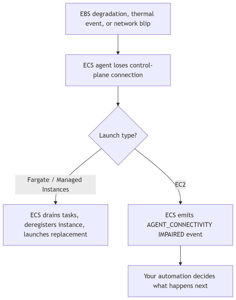
Here’s the detail worth sitting with. For Fargate and ECS Managed Instances, an impaired agent-connectivity check now triggers automatic recovery: ECS drains the running tasks, deregisters the instance, and launches replacement capacity on its own. That’s genuinely new. Previously, this failure mode needed the same manual detection loop no matter which compute type you were running. On EC2 launch type, you still get exactly that: an event, and the rest is on you.

The fork looks like this:

ECS node failure detection flow

Same trigger, same detection, two different endings depending on who owns the instance underneath.

If you already built the EventBridge-plus-Lambda pipeline for the old agentConnected flag, you can mostly retire that custom disconnect logic and key off AGENT_CONNECTIVITY instead. Same pattern, cleaner signal, one less bespoke piece of infrastructure to maintain.

Where I’ve seen this movie before

This is the same shape as EKS’s node monitoring agent, which has been turning kernel, storage, and network signals into Kubernetes node conditions and handing them to Karpenter for replacement since late 2024. ECS is arriving at the same idea from a different direction — a typed health signal a scheduler can act on, instead of a boolean you have to interpret yourself.

The gap is that EKS gives you this behavior on managed node groups and self-managed Karpenter too, as an add-on you install. ECS on EC2 still leaves you to wire the reaction yourself. I wouldn’t be surprised if that closes eventually — it’s an odd place to stop once you’ve already built the detection half.

What this doesn’t cover

This is infrastructure-layer health, not application health. A task can be serving broken responses just fine while its instance reports overallStatus: OK, because none of this looks inside your container. Keep your ALB target group checks and task-level health checks exactly as paranoid as they already are. This just catches the failures underneath them — the ones where the box itself stopped being trustworthy.

Worth doing this week

It’s free, and it’s already live in every AWS Commercial and GovCloud (US) region. If you’re on Fargate or Managed Instances, there’s nothing to configure — you already have it. If you’re still on EC2 launch type, this is a good afternoon project: point an EventBridge rule at AGENT_CONNECTIVITY IMPAIRED events and fold it into whatever already handles instance replacement, instead of waiting for someone to notice a node gone quiet.

EKS Finally Lets You Touch the Control Plane Knobs You’ve Been Faking with Workarounds

For years, running EKS meant accepting that the control plane was a black box you paid for but couldn’t tune. Want the scheduler to pack pods tighter to cut node count? Write your own scheduler plugin or run a second scheduler alongside the default one. Want HPA to react faster than the stock 15-second loop? You couldn’t — that number was baked into every managed cluster, full stop. Want shorter event retention so a CI-heavy namespace doesn’t bloat etcd? Not your call.

Control Plane configurable parameters

AWS announced in mid-August 2026 that this is no longer true. EKS now exposes a set of advanced configuration parameters across the scheduler, controller manager, and API server, set directly through CreateCluster and UpdateClusterConfig. No sidecar schedulers, no forked control plane, no support ticket asking AWS nicely. If you run a shared EKS platform serving multiple teams — which is exactly the kind of cluster where these defaults start to hurt — this is worth a proper look rather than a skim of the release notes.

What actually changed

Four parameters, across three components:

ComponentParameterRangeDefaultNeeds Provisioned Control Plane
kube-schedulernodeResourcesFit.scoringStrategyLeastAllocated, MostAllocatedLeastAllocatedNo
kube-controller-managerhorizontalPodAutoscalerSyncPeriod10s15s15sYes
kube-apiservereventTtl10m60m60mNo
kube-apiserverserviceNodePortRange10260327673000032767No

That’s a narrow slice of what upstream Kubernetes actually lets you configure, and I’d guess it stays narrow for a while — AWS is clearly starting with the parameters that are safe to expose without risking control plane stability, not opening the floodgates. Each one is set through a component-specific config block (kubeSchedulerConfig, kubeControllerManagerConfig, kubeApiServerConfig), works on Kubernetes 1.31+, and shows up in describe-cluster output along with every default you haven’t touched. Changes go through a rolling update of the control plane, so don’t expect them instant — budget a few minutes and poll with DescribeUpdate or aws eks wait cluster-active if you’re scripting it.

Scheduler: MostAllocated is the interesting one

This is the parameter I’d actually reach for first on a shared platform. By default, Kubernetes scores nodes with LeastAllocated, which spreads pods thin across your fleet so every node keeps headroom. That’s a reasonable default when you don’t know your workloads. It’s also exactly why clusters running steady-state services end up with fifteen half-empty nodes instead of ten well-used ones.

Switch to MostAllocated and the scheduler starts favoring nodes that are already carrying load, packing new pods onto them instead of spreading out. Combine that with Karpenter or Cluster Autoscaler consolidation and lightly used nodes actually get reclaimed over time — this is where the cost story lives, not in the scheduling decision itself.

You can also weight which resources drive scoring:

nodeResourcesFit:
  scoringStrategy:
    type: MostAllocated
    resources:
      - name: cpu
        weight: 1
      - name: nvidia.com/gpu
        weight: 100

Worth being precise here because the behavior is easy to misread. Weights are relative, not absolute — gpu: 100 next to cpu: 1 doesn’t mean CPU stops mattering, it means CPU only breaks ties once GPU availability is identical across candidates. The sharper gotcha is that omitting a resource from the list isn’t the same as giving it a low weight — leave memory out entirely and it’s excluded from scoring altogether, not just deprioritized. If you’re running mixed CPU and GPU node groups, that distinction is the difference between a config that behaves as intended and one that quietly ignores memory pressure.

Two things won’t change no matter which strategy you pick. First, the scheduler never moves pods that are already running — flipping the strategy only affects future placement, so if you’re trying to consolidate an already-packed cluster, you still need to evict or roll the workloads yourself. Second, filtering behavior is untouched; a pod that genuinely doesn’t fit on a node still won’t land there. And the honest trade-off with MostAllocated: you’re concentrating blast radius. Pack workloads onto fewer nodes and losing one of them, or an AZ event taking out a chunk of your fleet, now affects more pods per incident. On a cluster running twenty teams’ workloads, that’s not a hypothetical — I’d pilot this on a subset of node groups before flipping it cluster-wide.

HPA sync period: faster reaction, but only if you’ve earned it

Shortening horizontalPodAutoscalerSyncPeriod from the default 15 seconds down to 10 sounds like a free win — your workloads scale out sooner after a traffic spike. It isn’t free, and AWS gates it behind Provisioned Control Plane for a good reason: the HPA controller has to reconcile every HorizontalPodAutoscaler object in the cluster within that window, and shortening the window from 15s to 10s cuts the number of HPA objects your control plane can keep up with by roughly a third.

Here’s the part that’ll bite someone: EKS doesn’t validate the sync period against how many HPA objects you actually have. Set it to 10s on a cluster with more HPAs than that tier supports, and the update succeeds. Nothing errors. What happens instead is quieter and worse — some HPA objects stop getting reconciled on schedule, autoscaling starts responding slower than before you touched anything, and there’s no alarm or event telling you why. Before anyone on your team shortens this, run:

kubectl get hpa --all-namespaces --no-headers | wc -l

and check that number against your scaling tier’s supported count. If you inherit a cluster where someone already set this and autoscaling feels sluggish, that command is your first move, not a Datadog dashboard.

One more thing worth flagging to anyone managing the control plane scaling tier: once horizontalPodAutoscalerSyncPeriod is off default, you can’t move that cluster back from Provisioned to Standard mode. You have to reset the sync period to 15s first, then downgrade the tier. It’s a small detail, but it’s the kind of thing that turns into a surprised Slack message during a cost-optimization pass six months from now.

Event TTL and NodePort range: smaller blast radius, still worth reading the fine print

eventTtl is the simplest lever here — how long the API server holds onto Kubernetes events before deleting them, tunable from the default 60 minutes down to 10. On a cluster running CI/CD, batch, or AI workloads that generate thousands of events an hour, that’s real etcd pressure and real API server list latency you’re trimming. The catch: a shorter TTL only applies to events created after the change. Existing events keep whatever retention was active when they were written, so the storage benefit shows up gradually as the old events age out — not the moment UpdateClusterConfig returns. And once an event’s gone, it’s gone; if you lean on kubectl get events for postmortems, make sure something durable is already scraping events externally before you shorten this.

serviceNodePortRange is the one I’d reach for during a lift-and-shift rather than day-to-day tuning. Legacy apps that expect services on specific fixed ports outside Kubernetes’ default 30000–32767 window used to force a choice: rewrite the app, or bolt on a proxy. Now you can widen or shift the range (bounded to 1026032767, to stay clear of kubelet/kube-proxy health ports on the low end and the Linux ephemeral port range on the high end) and let the migrated app keep its original ports. Just remember it’s cluster-wide and non-retroactive — narrowing the range doesn’t kick out services already holding an out-of-range port, but recreating one of those services will fail to get that port back.

Where this actually earns a place in your platform

None of these four parameters change the availability or performance envelope of your control plane — AWS is explicit that clusters keep the same SLAs regardless. What they change is whether your platform team keeps working around upstream Kubernetes defaults with sidecar tooling, or just configures the thing directly and gets it recorded in CloudTrail like any other cluster change. On a shared EKS platform, the honest advice is: pilot the scheduler strategy on a low-risk node group first, treat the HPA sync period as something you validate with a headcount check rather than assume is safe, and use event TTL as a lever specifically for your noisiest CI or batch namespaces rather than a blanket cluster setting. Terraform and ACK support isn’t there yet — it’s Console, CLI, SDKs, CloudFormation, and CDK for now — so if your provisioning is Terraform-first, you’re looking at a temporary CLI-driven exception until that support lands.

The bigger signal here isn’t really any one parameter. It’s that AWS is starting to treat the EKS control plane as something you configure, not just something you consume. Worth watching what gets added to this list next.

Cell-Based Architecture on AWS, Part 6: Shipping Cells with IaC and ArgoCD

By this point in the series you’ve picked a partition key, chosen EKS or ECS as the substrate, worked out the networking, built in shuffle sharding and bake time, and made peace with what it all costs. What’s left is the least glamorous problem and the one that actually determines whether any of the above survives contact with a real team: how do you provision and update dozens of near-identical cells without dozens of near-identical ways for them to drift apart.

Shipping cells!

Infrastructure as code: the stamp pattern

The core idea is simple to state and easy to get subtly wrong in practice: write one module that describes a cell, and apply it once per cell with different inputs. A hands-on Terraform walkthrough of this pattern frames it as a blueprint you stamp out repeatedly, alongside a separately-built router layer that isn’t part of any individual cell’s module at all.

A minimal shape for that module looks something like this:

module "cell" {
  source   = "./modules/cell"
  for_each = var.cells

  cell_id       = each.key
  account_id    = each.value.account_id
  region        = each.value.region
  az            = each.value.az
  tenant_range  = each.value.tenant_range
}

variable "cells" {
  type = map(object({
    account_id   = string
    region       = string
    az           = string
    tenant_range = string
  }))
}

The detail that matters more than the module code itself is state isolation. Each cell’s Terraform state needs to be genuinely separate — a distinct backend key per cell, not just a shared workspace inside one state file — so that a plan or apply against cell-07 can’t accidentally touch cell-03. A shared state file for “all cells” quietly reintroduces exactly the coupling the whole architecture exists to avoid, just at the tooling layer instead of the runtime layer.

CDK works the same way conceptually, even though the syntax differs. AWS’s own reference implementation structures this as three separate stacks — one for shared ECR repositories, one for the routing components, and one for the cell blueprint, which gets deployed repeatedly, once per cell. Terraform, CDK, or CloudFormation, the stamp pattern is the same idea wearing different clothes.

A cell registry as the single source of truth

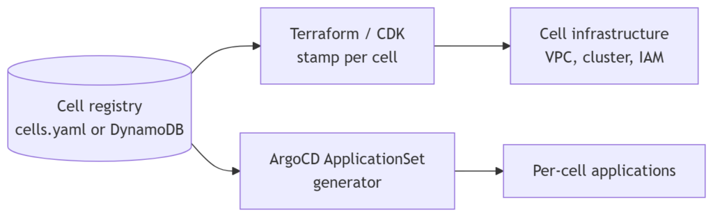
Once you’re past a handful of cells, you want one place that lists every cell that exists — its account, region, AZ, tenant range, and lifecycle status (active, draining, newly provisioned). This can be as simple as a cells.yaml checked into the same repo as your Terraform, or as robust as a DynamoDB table if other systems need to query it at runtime. What matters isn’t the storage mechanism, it’s that this registry becomes the one input that drives both your infrastructure provisioning and your application deployment generator — because the moment those two read from different sources of truth, you’ve created a gap where they can disagree about how many cells exist.

Cell registry

Deploying applications with ArgoCD

On the application side, ArgoCD’s ApplicationSet controller is built for exactly this fan-out. A list or git-file generator, sourced from the same cell registry, produces one child Application per cell (or per cell-and-app combination), rather than hand-maintaining one YAML file per cell per application.

apiVersion: argoproj.io/v1alpha1
kind: ApplicationSet
metadata:
  name: order-service-cells
  namespace: argocd
spec:
  generators:
    - git:
        repoURL: https://github.com/your-org/gitops-cells.git
        revision: main
        files:
          - path: "cells/*/registry.yaml"
  template:
    metadata:
      name: 'order-service-{{cell_id}}'
    spec:
      project: order-service
      destination:
        server: '{{cluster_endpoint}}'
        namespace: order-service
      source:
        repoURL: https://github.com/your-org/gitops-cells.git
        targetRevision: main
        path: 'apps/order-service/overlays/{{cell_id}}'

Platform-wide baseline components — an ingress controller, cert-manager, the monitoring agents every cell needs regardless of tenant — are a good fit for a separate App-of-Apps hierarchy, kept distinct from the per-cell, per-tenant applications so a change to the shared baseline doesn’t get tangled up with a single cell’s release train.

Sync waves are worth using deliberately here: router configuration and any cell-registration step should land before the cell’s own workloads sync, not after, or you risk a cell coming online with traffic already routed to it before its services exist. And each cell’s rollout should carry its own canary and bake time — tying back to the deployment discipline from earlier in this series — rather than one canary standing in for the whole fleet. A fleet-wide canary defeats the purpose of having cells in the first place; the point was that a bad release only ever touches one of them at a time.

The habit that actually keeps this from falling apart

None of this tooling prevents drift on its own. What prevents drift is treating the cell registry as a change that goes through the same pull request and review path as any other production change, and making sure both the Terraform plan and the ArgoCD ApplicationSet read from that same file. When someone adds cell-12 to the registry, that one commit should be the trigger for both the infrastructure to get stamped out and the applications to start deploying into it — not two separate manual steps that someone has to remember to keep in sync.

That’s really the throughline of this whole series. Cell-based architecture starts as a resiliency idea — smaller blast radius, contained failure — but by the time it’s running in production it’s mostly a delivery-engineering discipline. The isolation only holds up if your pipeline can safely stamp out cell N+1 in an afternoon, deploy into it with the same confidence as cell N, and tear it down just as cleanly if it turns out you didn’t need it. If your tooling can’t do that yet, the resilience story is still theoretical — and that’s a good place to start the next iteration of the design, rather than the last one.

Cell-Based Architecture on AWS, Part 5: Well-Architected and the Real Cost of Cells

Cell-based architecture gets pitched almost entirely as a reliability pattern, and it is one — the AWS Well-Architected Framework files it directly under the Reliability pillar’s bulkhead guidance. But it touches all six pillars once you actually build it, and at least two of them — cost and sustainability — tend to get discovered the hard way, after the architecture is already in production and the bill has arrived.

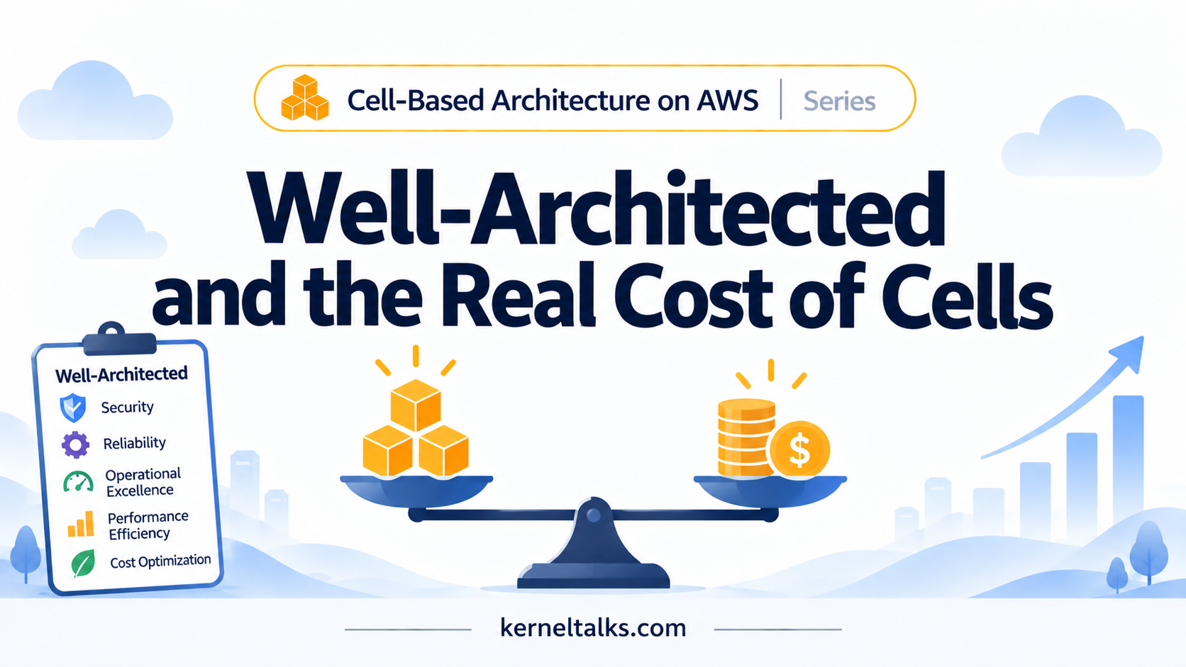
Well architected and cost in Cell Based Arch!

Running it through all six pillars

Reliability is the pillar cells were designed for, and it’s the easy one: smaller, isolated fault domains, contained blast radius, and a natural unit for fractional deployment.

Operational excellence cuts both ways. Cells give you a clean unit for canary releases and bake time, which is a genuine operational win — but every cell you add is another entry in the on-call runbook, another set of dashboards, another thing that can silently drift out of configuration with its siblings if your automation isn’t keeping up.

Security benefits in the same shape reliability does: a leaked credential or a misconfigured IAM policy inside one cell doesn’t automatically hand over the rest of the estate. The cost is that you now have N sets of IAM roles, N certificates, and N network boundaries to keep patched and rotated instead of one.

Cost optimization is where the trade-off gets sharp, and it’s covered in more detail below.

Performance efficiency tends to improve with smaller cells, because a noisy neighbor problem shrinks to the size of one cell instead of the whole platform. AWS’s ad-serving case is a clean illustration in the other direction: when tenants shared in-memory state on common infrastructure, one tenant with a large dataset could trigger memory pressure that degraded everyone sharing that heap, which is precisely the failure mode dedicated per-tenant compute was brought in to solve.

Sustainability is the pillar cell-based architecture can quietly work against. Fixed-cost resources replicated per cell — a NAT gateway sized for peak, a node pool that never scales below some minimum — sit idle a lot of the time by design, since isolation means you can’t pack unrelated tenants’ spare capacity together. Idle reserved capacity is wasted energy whether or not the AWS bill makes that obvious.

The cost math that catches people off guard

A few numbers are worth having in your head before you commit to a cell count.

An EKS control plane costs roughly $0.10 an hour, which works out to around $73 a month — and that’s before a single pod runs. Ten cell-per-cluster EKS deployments means roughly $730 a month in control-plane fees alone, on top of whatever compute those clusters actually run. ECS doesn’t have this problem in the same way — a cluster is a free logical construct, and billing starts at the task — which is a real reason cluster-per-tenant is a more forgiving pattern on ECS than on EKS.

AWS PrivateLink interface endpoints run close to $7.30 a month each plus data transfer, which is trivial shared once across a tier of cells and a real line item if you accidentally provision one per cell instead of pre-wiring it once at the tier level — the difference between those two choices is exactly what drove an 80 percent cut in network configuration overhead in AWS’s own ad-serving redesign.

And the starkest number in that same case study isn’t a unit price at all — it’s utilization. Before the redesign, the isolated-per-tenant fleet ran at roughly 3 percent average CPU and 19 percent average memory, with servers idle more than 98 percent of the time. That’s the cost of strict isolation taken to its logical extreme: every tenant’s capacity has to be sized for that tenant’s peak, and peaks, by definition, don’t happen most of the time.

Karpenter and the bin-packing tension

If you’re on EKS, Karpenter earns its cost savings mainly through consolidation — packing workloads onto fewer, better-utilized nodes and leaning on Spot capacity where it’s safe to. Karpenter documentation and the practical write-ups from teams running it at scale are consistent on this: it works best with a large pool of mixed workloads to bin-pack across dozens of nodes with varied sizes, not a handful of strictly-separated node pools each sized for one tenant.

Cell isolation deliberately works against that. If every cell gets its own NodePool to preserve the isolation boundary, you’re intentionally giving up some of Karpenter’s consolidation opportunity in exchange for the guarantee that one cell’s workload can’t crowd out another’s. That’s a legitimate, conscious trade — not a mistake — but it’s worth naming explicitly rather than discovering it as an unexplained line item during a cost review.

What this means for how you size cells

Everything above points back to the same conclusion from earlier in this series: start with fewer, larger cells, and shrink them as your tooling matures. A few practical habits follow directly from the cost picture:

  • Bundle genuinely fixed-cost resources — a VPC, a NAT gateway — across a batch of cells where the blast radius trade-off allows it, rather than one per cell.
  • Tier tenants by traffic profile instead of mapping every tenant to its own cell 1:1; group similar-sized tenants together and reserve full dedicated cells for the ones that actually need them.
  • Revisit your cell count and size against the AWS Well-Architected Tool and the SaaS Lens periodically — this isn’t a decision you make once and forget, it’s one that should move as your tenant mix and automation both change.

There’s no version of cell-based architecture that’s free. The honest framing is that you’re buying blast-radius containment with a mix of duplicated fixed costs, reduced bin-packing efficiency, and extra operational surface — and the job of a good design is making sure you’re paying for isolation you actually need, not isolation you inherited from copying someone else’s cell count. The last post in this series covers the part that makes all of the above sustainable day to day: provisioning cells with infrastructure as code and shipping application changes into them with ArgoCD.

Cell-Based Architecture on AWS, Part 4: Making Cells Actually Resilient

Splitting a system into cells doesn’t automatically make it resilient. If you still push a bad deployment to every cell at once, or if the same unlucky customer keeps landing on the same overloaded set of cells as everyone else, the isolation on your architecture diagram isn’t doing much for you in production. The pattern only pays off once you pair it with two more things: shuffle sharding, and real discipline about how changes roll out.

Resiliency in Cell Based Arch!

Shuffle sharding: spreading the overlap thin

Cells alone reduce blast radius by dividing customers into groups. Shuffle sharding goes a step further by giving each customer (or request) a near-unique combination of cells or nodes, so that any two customers only partially overlap, and the odds of two customers sharing the exact same full set of resources drop fast as your pool of cells grows. AWS describes this in more depth in Shuffle Sharding: Massive and Magical Fault Isolation, and the cell-based architecture FAQ is direct about the boundary: shuffle sharding works within a cell, but by definition a cell shouldn’t share state across cell lines, so don’t let shuffle sharding become an excuse to blur the boundary you just built.

The AZ-as-cell-boundary example from the Journey to Cloud-Native series makes the payoff concrete. With customers shuffle-sharded across three AZ-aligned EKS cells, a black-swan event that would have hit 100 percent of the application without cells is capped at roughly a third of capacity — and shuffle sharding also gives you a scaling lever for a single customer whose traffic spikes unexpectedly, since their load doesn’t have to be absorbed by one fixed cell.

Bake time and fractional deployment

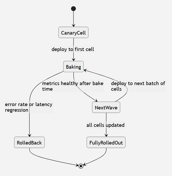
The other half of real resilience is how you ship changes. A cell-based system gives you a natural unit for fractional deployment — roll a change to one cell, watch it, then the next, rather than everywhere at once. What actually makes this work is bake time: a deliberate pause after each incremental step, long enough to know whether the change caused trouble before promoting it further. Depending on the system, that might be fifteen minutes or several hours — the right duration is whatever it takes for you to trust the signal, not a fixed number copied from someone else’s runbook.

The discipline that goes with it is equally important: roll back at the first sign the release is destabilizing things, rather than pushing forward hoping it stabilizes on its own. A fractional failure contained to one cell is a good outcome. A full rollout that later needs a full rollback is the outcome cells were supposed to prevent. Stateful changes deserve extra caution here specifically because they’re harder to walk back — a schema migration that can’t be un-run is a one-way door, cell-based or not.

Release Flow

AWS’s own hyperscale teams lean on progressive delivery tooling for exactly this — Argo Rollouts alongside EKS, watching response time and error rate as the promotion signal, described in the same Journey to Cloud-Native post. We’ll come back to wiring this into ArgoCD directly in the last post of this series.

Monitoring: per-cell, and in aggregate

Splitting one system into many cells multiplies your monitoring surface by the same factor. Each cell needs its own health signal — white-box metrics from inside the application, black-box checks from outside it, and business metrics that catch problems the infrastructure metrics miss entirely, like a quiet drop in successful checkouts. On top of that, you need an aggregate view that rolls individual cells up into “how many cells are healthy right now,” because a dashboard with forty individual cell panels and no summary is not a dashboard anyone can act on during an incident.

Tag everything with a cell identifier from the start — logs, traces, and metrics alike — so that when something does go wrong, correlating the failure back to a specific cell is a query, not an investigation. On EKS, Karpenter’s topology spread support and AWS’s Zonal Shift capability are worth pairing with AZ-aligned cells specifically, since they let you push pods away from an impaired zone and cordon affected nodes without hand-rolling that logic yourselves.

Multi-cell transactions: avoid them if you can

Sooner or later someone will ask for a request or a report that needs data from more than one cell. Handle this as a deliberate, external coordination step — a map-reduce-style service that calls each cell through its normal public interface, never by reaching into a cell’s internals directly — and treat every one of these you add as a real complexity cost, not a free feature. Each cross-cell dependency is a small crack in the isolation boundary you built the rest of this architecture to protect. Some are unavoidable. Most are worth pushing back on.

Resilience, in a cell-based system, isn’t a property you get from the architecture diagram. It’s the sum of a routing layer that fails safely, a shuffle-sharding strategy that keeps blast radius genuinely small, and a deployment process that treats bake time as non-negotiable. Get the diagram right and skip the process, and you’ve built an expensive way to still take a full outage. Next in the series: what all of this actually costs, and how it maps onto the Well-Architected Framework beyond just reliability.

Cell-Based Architecture on AWS, Part 3: Networking a Multi-Cell Estate

Every cell you design is, by intent, isolated from every other cell. The one piece of the system that can’t fully follow that rule is the network path that decides which cell a piece of traffic reaches in the first place. Get the routing layer wrong and you’ve rebuilt the single point of failure you were trying to eliminate — just one layer higher up.

Networking in Cell Based Arch!

VPC topology: per-cell, shared, or AZ-as-boundary

There’s no single correct way to lay out VPCs against cells, and the right answer depends on which boundary you’re actually defending. A VPC per cell gives the cleanest isolation — a NACL misconfiguration or route table mistake in one VPC can’t reach another — but it multiplies NAT gateways, VPC endpoints, and IP address planning by the number of cells you run. A shared VPC with dedicated subnets per cell is cheaper to run and easier on IP address management, at the cost of some shared blast radius at the VPC level itself.

A third option skips the VPC question and uses the Availability Zone as the cell boundary directly. AWS’s own Journey to Cloud-Native architecture write-up describes exactly this: pods aligned into cell groups on EKS, spread across three AZs, with only the routing layer — Route 53, DynamoDB, and the load balancer — shared across the whole system. The payoff is concrete: without cells, an initial bad event could take out the entire application; spread across three AZ-aligned cells, the worst case for that same initial hit caps at roughly a third of total capacity.

Whether you also want an AWS account as an isolation boundary is a separate, harder call. Multiple accounts contain the damage from leaked credentials or an account hitting a service quota, but account sprawl brings its own tax — every account needs to be onboarded into billing, monitoring, and security tooling, and that overhead doesn’t disappear just because Organizations makes account creation easy.

Route 53 weighted routing, worked through

For AWS-native cell routing, Route 53 weighted routing does a lot of the heavy lifting cheaply. Each cell (or infra group within a cell) gets a weighted alias record behind one stable DNS name, and adding capacity is just adding another weighted record — existing clients never need a DNS change. A record for a new cell might look like this:

{
  "Action": "CREATE",
  "ResourceRecordSet": {
    "Name": "orders.us-east-1.example.com",
    "Type": "A",
    "SetIdentifier": "cell-04",
    "Weight": 50,
    "AliasTarget": {
      "HostedZoneId": "Z35SXDOTRQ7X7K",
      "DNSName": "cell-04-alb.us-east-1.elb.amazonaws.com",
      "EvaluateTargetHealth": true
    }
  }
}

Turning on health evaluation matters here — it’s what keeps Route 53 from sending traffic to a cell whose ALB has gone unhealthy. A hosted zone supports up to 10,000 weighted records, so this scales to a lot of cells before you need to think about it again.

The ALB quotas that quietly cap your design

Two unglamorous Application Load Balancer quotas end up shaping infra-group size before any architecture diagram does: a maximum of 100 target groups per load balancer, and a maximum of 5 target groups per listener rule. Work through the arithmetic and one ALB, configured with reasonably granular listener rules, comfortably serves on the order of 50 tenant or cell targets before you need a second ALB — which is exactly the trigger AWS Ads used to decide when to add a new infra group rather than scale the existing one vertically. Knowing this number before you design the routing layer saves a redesign later.

PrivateLink for shared dependencies — and its cost

Cells rarely live in complete isolation from the rest of your platform; they usually need to reach a handful of centrally-owned services — a shared cache, an identity provider, a billing system. AWS PrivateLink is the standard way to expose those without opening them to the public internet or wiring up VPC peering per cell. The trick that actually pays off is pre-wiring the interface endpoints once, at tier or platform creation time, rather than per tenant — AWS Ads reports an 80 percent cut in network configuration overhead from doing exactly that. Each interface endpoint runs a modest, predictable cost — roughly $7.30 a month plus data transfer — which is close to noise once it’s shared across dozens of cells, and a line item worth tracking once it’s multiplied per cell instead.

Where a Transit Gateway shows up to connect layers of cells to each other, treat it carefully. A single TGW sitting at the center of every cell-to-cell path becomes exactly the kind of shared point of failure the whole architecture was designed to avoid. If cross-layer traffic is limited to a small, known set of backend cells, bilateral connections are often the safer default over a hub-and-spoke TGW.

Where VPC Lattice fits

Amazon VPC Lattice is worth knowing about for the service-to-service leg of this problem specifically. It gives services a logical, IAM-authorized identity instead of an IP address, and it works across EC2, ECS, EKS, and Lambda targets in different accounts and VPCs without hand-built peering or Transit Gateway routes. That makes it a good fit for the case where a cell’s workloads need to reach a small set of centrally-owned services elsewhere in the organization — but it’s not a cell router. It solves reachability between services, not the “which cell does this customer belong to” assignment problem, which still needs the DynamoDB-and-DNS pattern from the routing layer.

Certificates: the boring single point of failure

One detail that’s easy to skip and expensive to skip: give each cell its own TLS certificate with its own expiration date rather than sharing one certificate estate-wide. A single shared certificate that expires or gets misconfigured is a shared blast radius, no different in kind from a shared VPC route table — it just doesn’t look like one until it fails.

Networking is the layer of a cell-based system you actually want to be a little boring — predictable quotas, pre-wired connectivity, health-checked routing, and nothing clever sitting in the critical path that doesn’t need to be there. Boring networking is what makes the resiliency claims in the next post actually hold up under a real failure, rather than just on the architecture diagram.

Cell-Based Architecture on AWS, Part 2: EKS or ECS for Your Cells, and the Services That Hold Them Together

Once you’ve picked a partition key, the next decision is what actually runs inside a cell. For containerized workloads that’s an EKS-or-ECS question, and it’s worth more thought than “we already know Kubernetes.” The substrate decision determines how expensive isolation is per cell, and cost per cell is a number you’re about to multiply by every cell you’ll ever run.

When you have a choice to make!

EKS cells: namespace, or full cluster?

Inside EKS, a cell can live at two different depths. A namespace-per-cell model, with resource quotas and network policies enforcing the boundary, is cheap — one control plane serves every cell, and you’re mostly paying for the compute the pods consume. The catch is that the control plane itself becomes a shared blast radius domain again. A CRD conflict, an API server issue, or a cluster-wide add-on misbehaving can still touch every cell in that cluster, which undermines a chunk of the reason you wanted cells in the first place.

Cluster-per-cell removes that shared surface entirely, at a real price: an EKS control plane fee for every cluster, a separate node group or Karpenter deployment per cluster, and its own set of add-ons, IAM roles, and networking to keep patched. AWS’s own containerized cell-based reference design uses this model — pods are grouped into cell groups inside EKS, with topology-aware routing hints helping keep traffic within a cell’s Availability Zone rather than crossing between them. That Journey to Cloud-Native architecture post is worth reading end to end if you’re leaning EKS.

ECS cells: cluster-per-tenant is nearly free, until it isn’t

ECS clusters cost nothing to create — the meter starts when a task runs, which makes cluster-per-tenant a genuinely cheap way to get hard compute isolation without touching a Kubernetes control plane at all. It’s a well-worn SaaS isolation pattern for exactly that reason.

It’s also a pattern that can quietly become the problem. Amazon’s ad-serving platform ran an early cellular design that allocated a dedicated AWS account, Application Load Balancer, and ECS cluster to each tenant. Documented in AWS’s write-up on building hybrid multi-tenant architecture for stateful services, that setup hit real limits at a surprisingly small scale: just 18 clients spread across four AWS Regions already needed 181 separate targets to manage, onboarding a new client took roughly 52 days end to end, and average CPU utilization across the fleet sat around 3 percent. Strict isolation had bought accuracy, but the servers spent over 98 percent of their time waiting on requests that never came, because each tenant’s dedicated capacity had to be sized for its peak, not its average.

The fix wasn’t to abandon per-tenant isolation — it was to stop mapping tenants one-to-one onto cells. AWS Ads moved to a three-level hierarchy: a tier groups tenants with similar traffic profiles, a cell is the AWS account boundary within a tier, and an infra group — one VPC, one ALB, a set of per-tenant ECS clusters — is the reusable unit inside a cell. Onboarding became a configuration change against pre-wired infrastructure instead of a multi-week build, dropping to about 7 days. The lesson generalizes past ECS: your isolation boundary and your scaling unit don’t have to be the same thing.

The building blocks that show up in almost every cell design

Regardless of EKS or ECS, the same handful of AWS services tend to appear in the architecture diagram:

PurposeTypical service
Container computeAmazon EKS or Amazon ECS, often on Fargate or with Karpenter-managed EC2
Traffic routing to cellsAmazon Route 53 weighted or DNS-based routing, Application/Network Load Balancer
Cross-account, cross-compute service reachabilityAmazon VPC Lattice, AWS PrivateLink
Cell-assignment stateAmazon DynamoDB — fast, highly available, a natural fit for “which cell does this customer belong to” lookups
Container imagesAmazon ECR
Observability per cellCloudWatch Container Insights, Amazon Managed Service for Prometheus, Amazon Managed Grafana
Cost visibility per cell/tenantKubecost against Amazon Managed Prometheus for multi-cluster cost monitoring
DeploymentInfrastructure as code (Terraform or CDK) plus ArgoCD for the app layer

The DynamoDB piece deserves a callout. AWS’s own hyperscale teams have mapped customers to cells with a hash function whose result is stored in DynamoDB, precisely because that table needs to answer “which cell?” reliably under load without becoming a bottleneck itself. It’s a small, boring piece of infrastructure carrying an outsized amount of trust.

Router patterns, briefly

Every design needs something that decides which cell a given request goes to, and there are three broad ways to build it, each with a different failure profile. A load-balancer-style router sits in the request path permanently, forwarding every packet — simple for clients, but now in the critical path for every transaction. A hand-off router authenticates the client once and returns the cell’s address, after which the client talks to the cell directly; this removes the router from the ongoing request path but pushes some logic into the client. A DNS-based router leans entirely on the DNS system’s own reliability, at the cost of DNS-level control over routing decisions. None of these is strictly better — which one fits depends on how much control you need over routing versus how simple you want the client side to be. We’ll dig into this properly, including where a control-plane/data-plane split helps, in the networking post.

Which one would I reach for

If I’m starting fresh on containers and the workload doesn’t need OS-level tuning, I lean ECS cluster-per-cell for the early cells. It’s cheaper to stand up and tear down, and the limits you bump into are AWS service quotas rather than Kubernetes control-plane behavior you have to reason about separately. I’ll reach for EKS cluster-per-cell once the team already runs Kubernetes elsewhere and wants one operational model across cell and non-cell workloads — the consistency is worth the extra control-plane bill at that point. Namespace-per-cell inside a single EKS cluster is the one I’d be most cautious about recommending for anything claiming strong isolation; it’s cheap, but you’re still betting the whole cluster’s control plane won’t be the thing that takes every cell down at once.

The substrate decision sets your cost floor. The networking layer sets your failure floor — which is where we’re headed next.

Cell-Based Architecture on AWS, Part 1: The Thought Process Before You Draw a Single Box

A dropped table. A malformed feature flag. A load balancer configuration that fails open instead of closed. None of these need a regional outage to hurt you. They only need a blast radius big enough to reach every one of your customers at once. Multi-AZ and multi-Region deployments protect you from AWS having a bad day. They do nothing for the day your own deployment pipeline has one.

Where it begins!

That gap is what cell-based architecture is built to close, and it’s the reason AWS has used the pattern internally for over a decade before writing it down as public guidance. Before touching a Terraform file or an EKS console, the job is mostly a thinking exercise: deciding what a “cell” is for your system, what goes inside one, and how big is too big. Get that wrong and no amount of Kubernetes or containers expertise will save you later.

What a cell actually is

A cell-based architecture partitions a system into a set of independent, self-contained replicas, each serving only a slice of the overall client base. AWS’s guidance on reducing scope of impact with cell-based architecture frames this as an extension of the same fault isolation AWS already applies at the Availability Zone and Region level, just moved down into your own workload.

The two things that make a cell a cell, rather than just another replica behind a load balancer, are isolation and partitioned state. Every cell runs standalone, with no runtime dependency on any other cell, and the data it owns isn’t replicated elsewhere. A thin routing layer is the only thing that knows all the cells exist — clients (or their traffic) get assigned to exactly one cell and stay there. AWS’s cell-based architecture guidance on GitHub puts it plainly: if a bad actor or a bug wipes a database inside one cell holding a tenth of your users, you’ve lost a tenth of your data, not all of it, and you can restore a tenth of a database a lot faster than the whole thing.

This is also why it sits inside the Reliability pillar of the AWS Well-Architected Framework, specifically as an expanded form of the bulkhead architecture best practice. It’s explicitly called out as guidance for workloads that need extreme levels of resilience, not a default starting point for every workload you own.

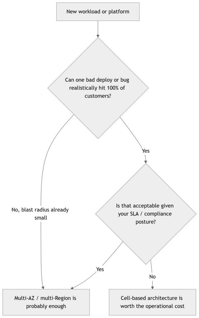
Decision flow for Cell Based Arch!

Where cell boundaries come from

The first real decision — before compute, before networking — is the partition key. What is the unit of the system that gets isolated? Tenant ID, customer account, geography, and traffic tier are the usual candidates, and the choice cascades into everything downstream: how routing state is modeled, how the data layer gets sharded, and later, how your Terraform and GitOps repos get structured. Pick this wrong and you’ll be re-partitioning a live system later, which is exactly the kind of one-way-door change the whole pattern is meant to avoid.

The second decision is where the isolation boundary actually sits. An AWS Availability Zone can be the cell boundary, as AWS’s own architecture teams have done for containerized workloads. An AWS account can be the boundary, which limits blast radius from compromised credentials or account-level service quotas, at the cost of more accounts to govern and bill. Or the boundary can sit lower, at the Kubernetes namespace or ECS cluster level, inside a shared account. None of these is universally correct — it depends on what failure you’re actually trying to contain.

Sizing cells: the trade-off nobody gets to skip

Smaller cells reduce blast radius, since each one carries fewer customers. They’re also easier to test, easier to reason about, and individually simpler to operate. But more cells means more of everything else — more routing entries, more monitoring dashboards, more deployment pipelines running in parallel — and that operational surface area doesn’t shrink just because each cell is small.

Larger cells go the other way. Fewer moving parts, better economics per customer, less to monitor — and a bigger blast radius when something does go wrong inside one. There’s no formula that spits out the “right” cell size; it’s a genuine trade-off, and the common pattern is to start with a small number of large cells and shrink them over time as your automation and tooling mature enough to absorb the extra operational load. Jumping straight to hundreds of tiny cells before your deployment tooling can handle it just moves the failure mode from “blast radius” to “operational chaos.”

Is this even the right tool for your workload

Here’s the opinion part: most teams don’t need this. If you’re running a single EKS cluster for an internal tool with a handful of customers, cell-based architecture will cost you more in engineering time than any outage it prevents. It earns its place when a single failure hitting all customers simultaneously is genuinely unacceptable — hyperscale SaaS, regulated industries with strict blast-radius requirements, or platforms where a black-swan event (a sudden traffic spike from one tenant, a bad config push, a compromised credential) has to be contained by design, not by hoping your canary process catches it in time.

A planning checklist before you open the AWS console

  • Identify the partition key your cells will be organized around.
  • Decide the isolation boundary: namespace, cluster, Availability Zone, or AWS account.
  • Decide where cell-assignment state lives and who owns the routing layer.
  • Decide which resources are centralized (accepting shared blast radius) versus replicated per cell (accepting cost).
  • Set an initial target cell size, and the trigger condition for splitting or adding another one.

That last point matters more than it looks. Without an explicit trigger — a tenant count, a request-rate threshold, an AWS service quota you’re approaching — cell sizing decisions get made reactively, usually during an incident, which is the worst possible time to be making them.

The rest of this series works through the pieces that hang off these decisions: which AWS container services and building blocks actually implement a cell on EKS or ECS, how the networking layer routes traffic without becoming a single point of failure itself, how shuffle sharding and deployment discipline make the isolation real rather than theoretical, what this costs against the Well-Architected pillars, and how to provision and deploy dozens of these things without losing your mind. Next up: choosing between EKS and ECS as your cell’s compute substrate.

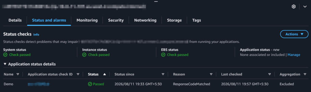
Amazon EC2 Application Status Checks: A Native Health Check for the Application Layer

An EC2 instance can show 2/2 status checks passed while the application on it has been dead for twenty minutes. The hypervisor is fine, the kernel booted, the network stack answers pings — none of which tells you whether nginx stopped accepting connections or your app is stuck returning 500s to every request. That gap, between “the instance is up” and “the thing running on it actually works,” is what application status checks now cover natively, as of August 10.

EC2 Application Status Checks!

The Gap It Fills

EC2 has run two automatic checks on every instance for years: a system status check watching the AWS hardware underneath, and an instance status check watching the guest OS and its network config. An attached EBS check came later for volume reachability. All three are automatic — you can’t turn them off or point them anywhere — and none of them look inside the application. A crashed worker process or a web server that stopped listening is invisible to EC2, because the instance itself still looks perfectly healthy.

Closing that gap used to mean building it yourself: an ALB target group health check if you had a load balancer, a cron job and a custom CloudWatch metric if you didn’t. Application status checks are AWS’s native answer to the second case, a fourth, opt-in check that speaks HTTP directly to your application.

How It Works

You define a check with a protocol (HTTP or HTTPS), a port, a path, and a status code matcher — the same shape as an ALB health check. Associate it with instances by ID or by tag, including aws:autoscaling:groupName to cover an entire Auto Scaling group in one call, and EC2 pings that port and path every 60 seconds. Fixed interval, no faster, no slower.

aws ec2 create-application-status-check \
    --protocol https --port 443 --path "/health" \
    --status-code-matcher "200"

Two consecutive failures flip the check to impaired, two successes flip it back to ok, both configurable, along with a 6-second timeout and a 300-second grace period after launch so a slow-starting app doesn’t get replaced before it’s ready. Set that grace period too low and Auto Scaling will happily replace instances that just needed more time to boot. Full parameter reference is in the Amazon EC2 User Guide.

Where the Checks Actually Run

Worth knowing before you roll this out: check traffic doesn’t come from some anonymous AWS endpoint. AWS provisions a managed network interface inside your own VPC, one per subnet-and-security-group combination, and traffic runs from within your VPC over AWS’s internal network, never the public internet. That managed ENI doesn’t count against your instance’s ENI limit, but it does count against your account’s ENIs-per-VPC quota, worth checking before a fleet-wide rollout across a lot of subnet-and-security-group combinations.

Check flow

The step people miss: CloudWatch gets a metric per check plus one aggregate per instance, and it’s only the aggregate that Auto Scaling watches. You can also specify the source subnet and security group yourself instead of letting AWS choose, useful if your network has segmentation rules a security review would care about.

App status check details

Auto Scaling, and the Deploy Trap

Auto Scaling groups already pull health signals from EC2, ELB, VPC Lattice, EBS, and custom checks. Application status checks slot in as one more. Associate the check with the group’s instances, and Auto Scaling replaces anything reporting impaired — no extra configuration needed. This earns its keep most on workloads that never sat behind a load balancer at all: backend workers, queue consumers, anything that never had a native AWS health signal before.

The catch: a deployment or restart makes the check fail too, since the app genuinely isn’t answering for a few seconds. Auto Scaling can’t tell “expected restart” from “actual crash,” so an unplanned deploy across a fleet can trigger a replacement storm you caused yourself. AWS gives you three ways to prevent that:

ApproachWhen to use it
Suppress the checkA known, bounded maintenance window
Exclude from aggregationValidating a new check without risking replacements
DisassociatePermanent removal

For routine deploys, automate suppression from your pipeline’s pre- and post-deploy hooks:

aws ec2 enable-application-status-check-suppression \
    --instance-ids i-0123456789abcdef0 --duration-seconds 3600

Put this in the deployment runbook before you need it, not after Auto Scaling has replaced half a fleet mid-release.

Two Gotchas Worth Knowing

When a check fails, look at the reason code before touching application logs. Redirects are a common false failure: health checks don’t follow 301s or 302s, so a /health path that redirects will fail unless you add that code to your matcher. Two other behaviors catch people off guard. The health check goes out over HTTP/2, so a minimal server that only speaks HTTP/1.1 in cleartext can fail a check that a plain curl would pass. And the HTTPS check never validates the server’s certificate, so a passing check tells you nothing about certificate validity.

What It Costs

Pricing: $0.01 per hour per managed ENI, per Availability Zone, plus standard CloudWatch pricing for the metrics. That cost tracks unique subnet-and-security-group combinations, not instance count. One Auto Scaling group in one subnet is one ENI per AZ, essentially free. A fleet spread across many subnets for segmentation reasons will rack up more ENIs than the instance count suggests, so it’s worth estimating that number before assuming this costs nothing. Default account quotas (50 checks, 5,000 targets) are generous for most teams and adjust automatically except for the targets limit, which needs a manual request.

Where This Fits

Application status checks aren’t a replacement for real observability. There’s no tracing, no latency data, just “did this path return the code I said meant healthy.” What they replace is whatever duct tape your team already built to answer that one question: a cron job and a custom metric, a sidecar pinging itself, a script from years ago nobody wants to touch. If that’s your current setup, especially for anything that doesn’t sit behind a load balancer, it’s worth an afternoon to pilot this with the check set to excluded before it can page anyone.